sviewgui is a PyQt5-based GUI for data visualisation of csv files or pandas.DataFrame objects. Main features:

Scatter, line, density, histgram, and box plot types

Settings for the marker size, line width, number of bins of histgram, color map (from cmocean)

Save figure as editable PDF

Code of the plotted graph is available so that it can be reused and modified outside of sviewgui

All graphs that sviewgui can generate is based on matplotlib.

 Usage

Here is a sample code. sviewgui has only one function 'buildGUI()', which starts the GUI. If you already have a CSV file that you want to look at, you can build the following code without any argument.

from sviewgui import sview as sv

# sample code 1
sv.buildGUI()

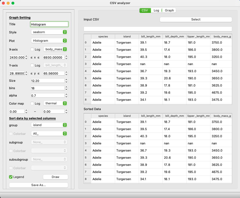
If you build this code, GUI window like the photo bellow will open.

Then, you can open your CSV file from the 'select' button.

Alternatively, you can also open the GUI using the file path or pandas' DataFrame object. Here is another sample code using Iris dataset.

import pandas as pd
from sklearn import datasets
# Sview-GUI
from sviewgui import sview as sv

# load iris
iris = datasets.load_iris()
# Create DataFrame object
df = pd.DataFrame(iris.data, columns=iris.feature_names)
df['target'] = iris.target_names[iris.target]

# export DataFrame as CSV file.
SAVE_PATH = 'data/dst/iris.csv'
df.to_csv(SAVE_PATH) # save as CSV

# build GUI with the filepath
sv.buildGUI(SAVE_PATH) 

# build GUI with pandas' DataFrame object
sv.buildGUI(df)

Then, let's build GUI with iris dataset.

You find that a table of iris dataset is displayed at the upper-right side of the GUI window.

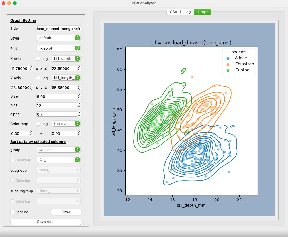
If you go to the 'Graph' tab, or if you scroll the left 'Graph Setting' panel downword and push the 'Preview' button, you can display the graph.

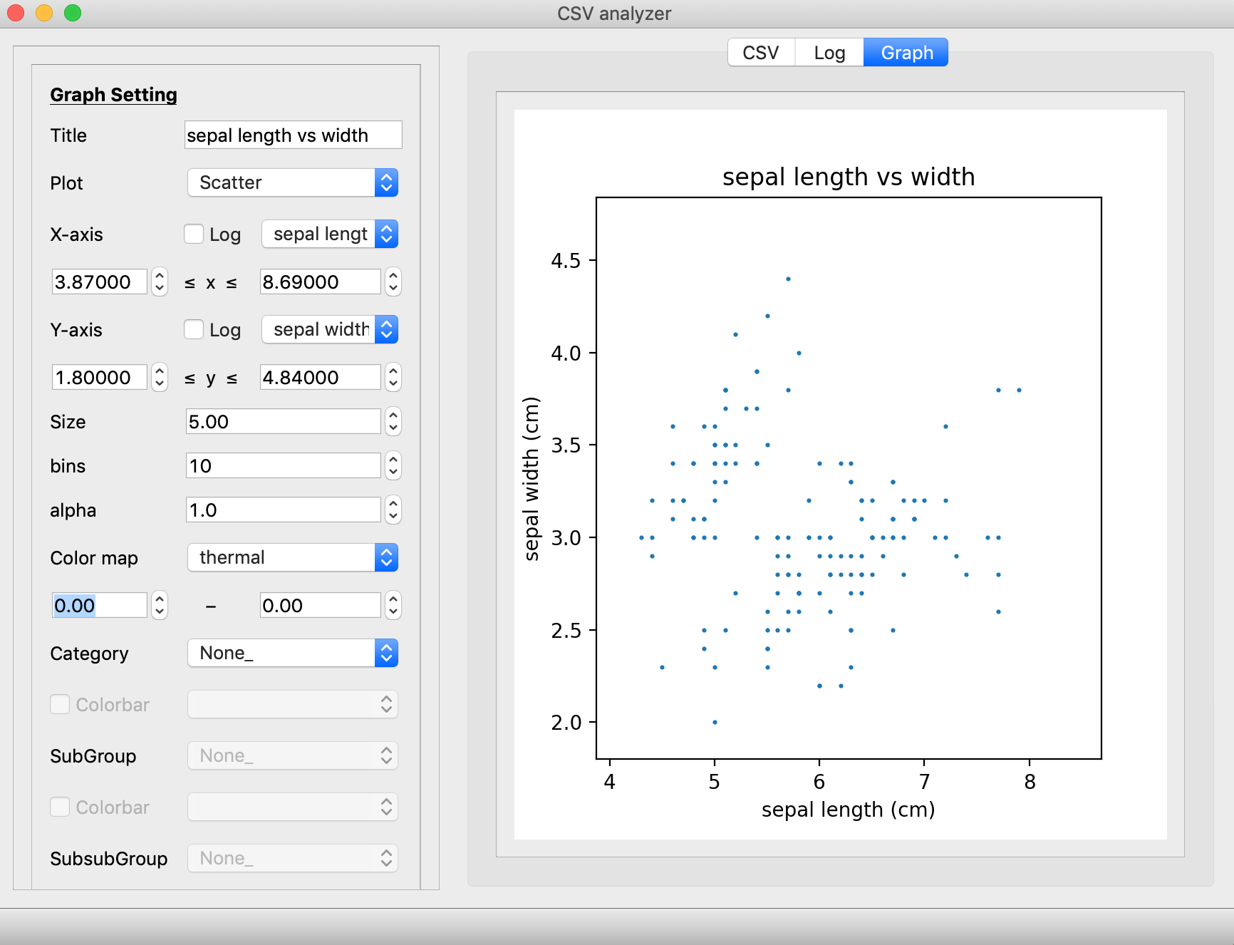
Most of the setting options are straight manner. From the top,

Title: title of the plot

Plot: Scatter, Density, Histogram, Line, and Box plot

X- and Y-axis: data and range of axes

Size: size of the markers of scatter plot or line width of line plot

bins: number of bins of Histogram

alpha: opacity of the plot

Color map: you can choose colormap from cmocean. Also you can set the range of colormap

Category, Sub- and Subsubgroup: You can choose the data by which you want to classify or sort the dataset on the plot

Colorbar: When you choose the data that is composed of numerical elements, you can choose whether you apply different color to each element, or colormap to the whole range of the dataset with colorbar

Legend: you can add legend (sorry for that you cannot adjust the position or size of legend yet, but hopefully in next update!)

Preview: display the plot

Save As...: you can save the plot as image (editable PDF)

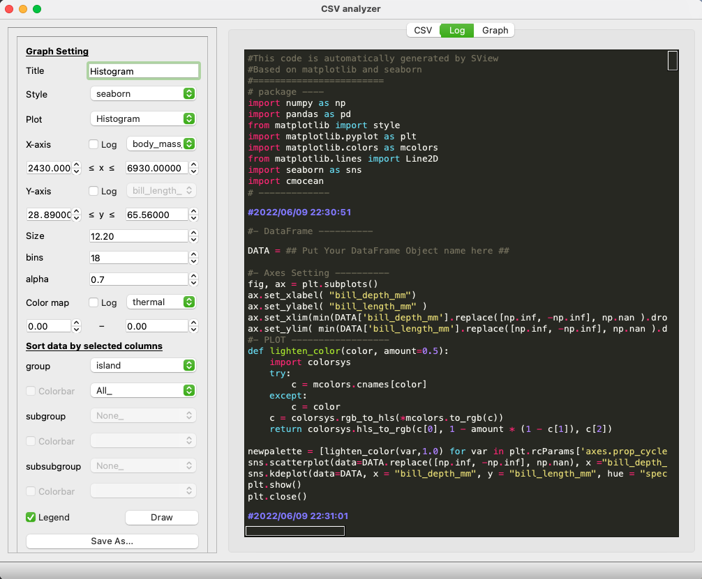
Log tab preserves the source code of the all graphs that you displayed at 'Graph' tab.