efshape is a python package for shape analysis of 2D image. The method is based on the combination between ‘Elliptic Fourier Analysis (EFA)’ and ‘Principal Component Analysis (PCA)’ and is called EF-PCA method.

The basic idea is to convert a 2D closed contour into a numeric dataset by EFA and then, using multivariate analysis (PCA), detect the major shape variation of the dataset. EFA enables you to describe the complicated shape complehensively as a number of dataset called elliptic Fourire descriptors (EFDs). One of the merits of this method is that you can easily reconstruct the shape from the descriptors, which also make it easier to interpret the shape variation of detected principal component axes.

In this package, you can choose three different types of EF-PCA methods: one of which, EFD-based EF-PCA, is suitable for directional object like bio-forms, and the others, Amplitude- and FPS-based EF-PCA, are suitable for non-directional object such as sedimentary grain. This package provides you both CUI- and GUI-based package.

 EF-PCA method

Elliptic Fourier Analysis

As mentiond above,the basic idea of EF-PCA method is converting shape into a number of numerical dataset and summarising those dataset by mutivariate analysis.

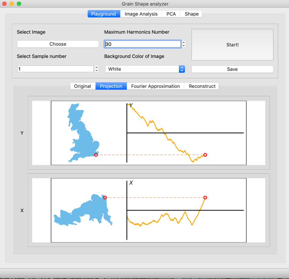
Elliptic Fourier Analysis is the method to convert the 2D shape into a set of numerical dataset (Kuhl & Giardina, 1982) . Let's imagine a closed contour and a moving point along the contour with a constant velocity. You can obtain the shape information as two periodic functions by plotting the $X$ and $Y$ coordinates of the moving point against time.

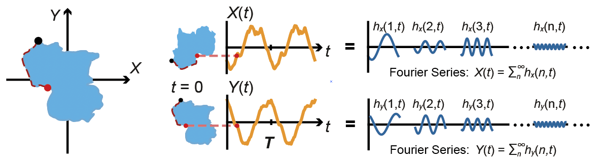
These periodic functions can be approximated by Fourier series.

$ \begin{align} X(t) &\simeq \sum_{n=1}^N a_n \cos (\frac{2n\pi t}{T}) + b_n \sin (\frac{2n\pi t}{T}) \label{x-coord} \\ Y(t) &\simeq \sum_{n=1}^N c_n \cos (\frac{2n\pi t}{T}) + d_n \sin (\frac{2n\pi t}{T}) \label{y-coord} \end{align}$.

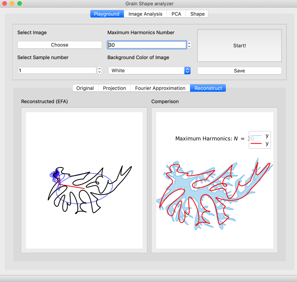
In these equations, the four coefficients, $a_n$, $b_n$, $c_n$ and $d_n$, are the unique parameters that determine the shape features and called Elliptic Fourier Descriptors (EFDs). $N$ is the maximum frequency number of Fourier series. Theoretically, as $N$ increases, the shape reconstructed by Fourier series will be more accurate and when $N$ goes infinity, the reconstructed shape will be exactly the same shape as original one. However, due to the limitaiton of original image's resolution, even if you choose huge $N$, the higher frequencies of Fourier series only provide the meaningless noise, which could badly affect the later analysis.

EFDs are multiple sets of numerics and it is difficult to interpret the meaning of each value. To make it simple, let's convert the Eq. ($\ref{x-coord}$,$\ref{y-coord}$) to matrix form.

\begin{align} &\begin{bmatrix} X(t)\\ Y(t) \end{bmatrix} \simeq \sum_{n=1}^N {\bf H}_n \\ &{\bf H}_n = \begin{bmatrix} a_n & b_n \\ c_n & d_n \end{bmatrix} \begin{bmatrix} \cos \left( \frac{2n\pi t}{T} \right) \\ \sin \left( \frac{2n\pi t}{T} \right) \end{bmatrix} \end{align}

Since each ${\bf H}_n$ is a formula of ellipse, it is called Harmonics Ellipse. The size of each harmonic ellipse can be interpreted as the amount of shape information of different scale of surface roughness.

To understand the actual meaning and get a sense of these harmonic ellipses, let's visualise how each ellipse affects the shape. Following two GIF animations shows the examples of shape reconstruction using the UK main island. The left figure shows the example with $N=3$ and the right figure is $N=20$.

Each harmonic ellipse is moving along the pre-number harmonic ellipse with different speed. For instance, the 3^rd harmonic ellipse goes around the 2^nd harmonic ellipse twice, while the 2^nd harmonics ellipse goes around the 1^st harmonic ellipse only once. If you look at the term inside of sin and cos term, you can find that the frequency of each ellipse is $n/T$, which means that each ellipse represents the different scale of surface roughness.

How many harmonic ellipses are suitable for shape analysis?
It is a bit difficult question but, theoretically, you cannot compute ellipses more than the half of the total number of coordinates of contour. This theoretical limitation determine the upper limit of the frequency of harmonics, which is called 'Nyquist frequency'. Further, even if $N$ is lower than the Nyquist frequency, in most cases, first several frequencies are enough to describe shape and higher frequency could often be a cause of error due to the various reasons such as the distortion of the photo, the condition of the sample and uncertainties caused by degitization processes. The amount of information that each harmonic ellipse has can be evaluated by Fourier Power Spectra (FPS) which is given by

\begin{align} {\rm FPS}_n = \frac{a_n^2 + b_n^2 + c_n^2 + d_n^2}{2}. \end{align}

One of the way to determine the number of frequency you use for the analysis is that calcurate the all FPS values of each frequency up to the Nyquist frequency, and then, choose the frequency where the cumulative FPS value exceed a specific threshold like 95% of total cumulative value (e.g. Costa et al., 2009).

In short, EFA converts the shape into a set of numerics called EFDs, each set of which describes the different scale of surface roughness and called Harmonic Ellipse. After EFA, you will obtain $4N$ EFDs. Thus, if you use 20 different frequencies, the target shape is described as 80 parameters for each sample.

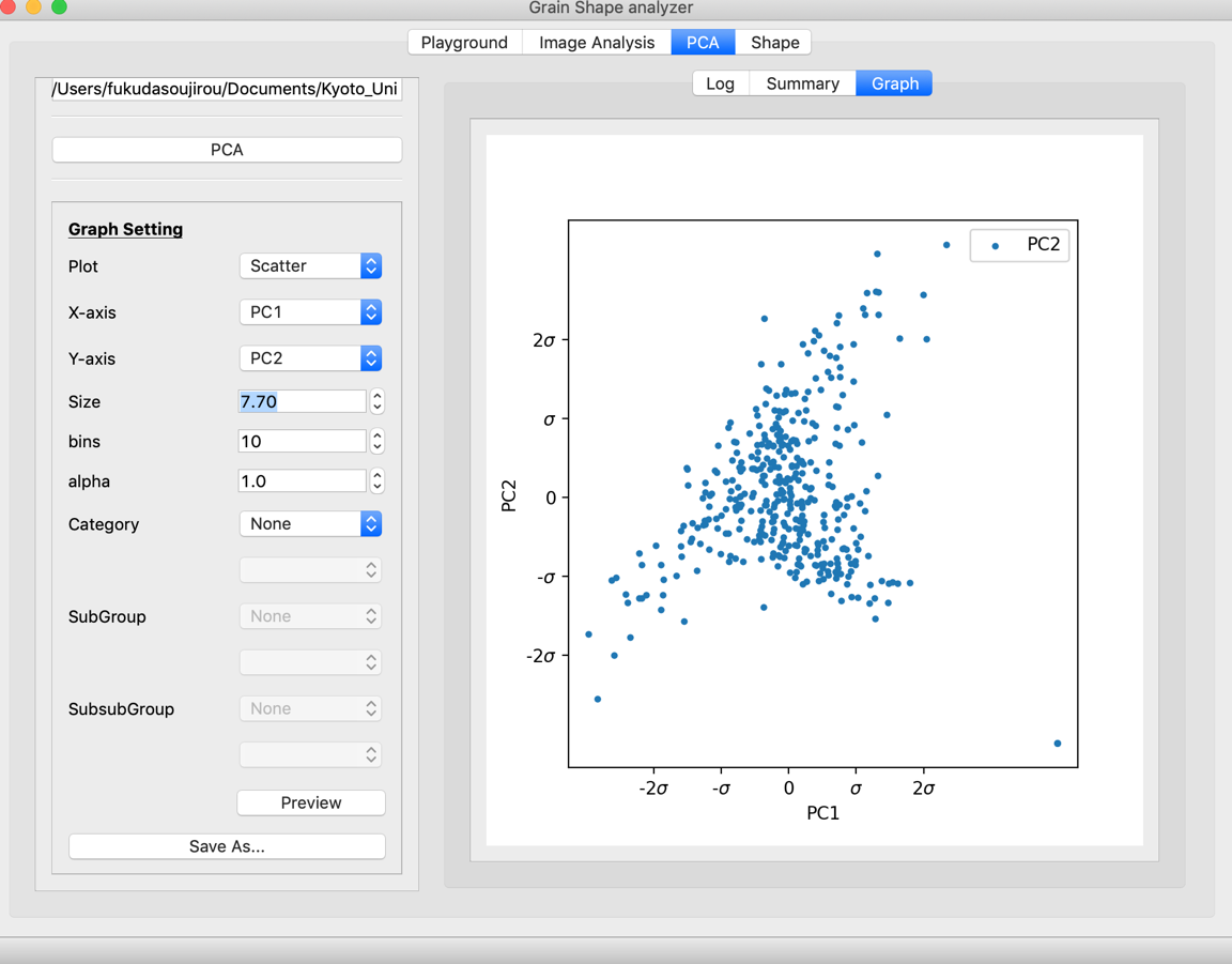
Principal Component Analysis

Principal Component Analysis (PCA) is one of the most basic multivariate analyses. PCA is a kind of coordinate transformation. PCA transforms the original multi-dimensional coordinate system to a new system in the way that your data has the biggest deviation on the first axis of new coordinate system and has the second-biggest deviation on the second axis. By doing so, you can reduce the number of dimension by neglecting the some of the last axes that less describe the variation of dataset in new coordinate system. Generally, first few new axes (called Principal Components: PCs) describes the large portion (e.g. more than 90%) of the variation of your dataset.

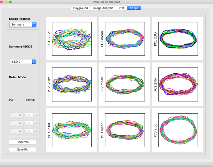
What PCA does in EF-PCA method is to detect the major shape variation to visualise the shape space.